In physics, angular momentum is a kinematic property of a system consisting of one or more point masses. Its importance derives from the fact that it is conserved in several physical circumstances, notably for objects in field-free space and for central-symmetric interactions. (Recall that a conserved property of a system is one that does not change over time.)
Before the advent of quantum mechanics, angular momentum did not play an important role in physics, as is witnessed by the 450 page book of Whittaker[1] in which three and a half page is devoted to it and the index contains only one reference to angular momentum.
Cajori, in his well-known history of physics[2] gives exactly half a line to the conservation of angular momentum. Since angular momentum is of great importance in quantum mechanics, post quantum mechanics texts on classical mechanics pay much more attention to it. For instance Goldstein[3] has about 25 entries in its index and about a fifth of his book devoted to it. See this article for the definition and role of angular momentum in quantum mechanics.
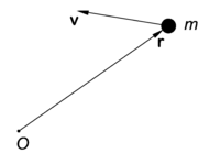
PD Image Point mass
m with velocity
v has angular momentum
L ≡
m r ×
v with respect to
O.
L is a vector pointing towards the reader, perpendicular to the plane of drawing, which is spanned by
r and
v.
Definition
The angular momentum of a single point mass m is defined with respect to a point O. Denote the vector from O to m by r (see the figure). Let the mass have velocity v, then
the angular momentum L of the point mass is defined as the cross product,

It follows from the definition of cross product that the vector L is perpendicular to the plane of the figure and points towards the reader. Note that the definition p ≡ m v for the linear momentum is introduced here.
The definition of the angular momentum of a system of n point masses is the following simple generalization:

Conservation of angular momentum
For simplicity we consider first the case of one point mass, generalization to n point masses is straightforward. The following important result will be proved: a particle that moves in a central-symmetric potential has a conserved angular momentum.
Using Newton's dot (fluxion) notation for time derivatives, we find

Use

where we invoked Newton's second law
 Hence the time derivative of the angular momentum is equal to the torque N,

It follows that the angular momentum is conserved—i.e., its time derivative is zero—if the applied torque N is zero, which means that either F is zero, or r and F are parallel, because in that case the cross product vanishes.
The former case (F = 0) occurs when the mass moves uniformly in homogeneous space (no external forces). Then also the linear momentum of the point mass is conserved, and therefore one rarely considers the angular momentum in the case of uniform rectilinear motion.
The second case (r parallel to F) is more interesting. In order to see what this means for the potential, we must assume that F is conservative, i.e., its curl vanishes, otherwise the potential cannot be defined. If F is conservative,
then F is minus the gradient ∇ of a potential V(x,y,z),

so that for a conservative force the torque is

The quantity in brackets is known in group theory as a Lie derivative of the full rotation group SO(3). In quantum mechanics it is a well-known operator, namely the orbital angular momentum operator (except for the factor  ).
).
From the general properties of Lie derivatives—or equivalently orbital angular momenta—it follows that the torque vanishes whenever the potential V(x,y,z) is rotationally invariant (also known as an isotropic or central-symmetric potential). This means that the function V(x,y,z) depends on r only, when expressed in spherical polar coordinates (r, θ, φ).
We can prove the vanishing of the torque more explicitly by expressing the gradient ∇ in spherical polar coordinates and writing the cross product as a determinant, using that the derivatives of V with respect to θ and φ are zero,

Note that the third member in this equation shows that r (the second row) and −F (the third row) are indeed parallel to each other in the case of an isotropic potential. Both vectors possess only a radial coordinate; r by definition and F because the gradient of V has only one non-vanishing component, the radial component.
A well-known example of a system with conserved angular momentum is the earth orbiting the sun. To a very good approximation the gravitation is central-symmetric (rotationally invariant) and hence the earth's orbit is characterized by a conserved angular momentum, i.e., the time derivative of the angular momentum (torque) is zero. Kepler's second law is a direct consequence of this conservation of angular momentum.
Extension to n point masses
When in a system of n point masses the particles do not interact mutually, the extension is simply:

where the forces F i are external. If the total external torque is zero, the total angular momentum of the system is conserved.
When the particles do interact, i.e., there are non-zero internal forces, then the result still holds, provided the internal forces are central-symmetric and additive. No internal torque occurs in that case. In order to show this, we recall that Newton's third law (action = −reaction) holds for central-symmetric forces. Indicating internal forces by a double suffix, we write Newton's law as follows,

where the left hand side is the force on particle i executed by particle j and the right hand side is i acting on j. Both forces act along the vector pointing form particle i to j,

so that

where

The total internal torque on particle i is,

Under assumption of additivity, the total internal torque can be written as

and

where F i (characterized by a single suffix) is external.
Separation of center of mass
The angular momentum of a system of point masses with respect to an arbitrary point O can be separated into two terms. The first term is the angular momentum with respect to O of a fictitious particle with total mass M positioned at the center of mass C of the system. The other term is the sum of the angular momenta of the particles with respect to C.
The center of mass C is determined by

Introduce s i for particle i at point P i

Note that

and hence also

The two cross terms in the following equation vanish and the two diagonal terms are non-vanishing,

The two remaining terms are:

If the total system moves in homogeneous (field free) space, the first term is conserved and is usually not of much interest. The second term, the sum of the angular momenta of the n particles with respect to the center of mass, is usually designated the total angular momentum of the system,

where the position vectors s i are defined with respect to a system of axes with origin in the center of mass C of the system.
Circular motion around a fixed axis
A system often encountered in physics is a particle (point mass) that moves along a circle in a fixed plane. Let us choose a system of axes such that the plane of motion is the x-y plane, with the z-axis perpendicular to the plane.
The coordinates of the particle and its time derivative are

where we used that the radius r of the circle is time-independent. The angular momentum is given by

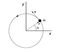
Point mass
m moves counterclock-wise on a circle. Instantaneous velocity
v is tangent to the circle. Angular velocity and angular momentum point toward the reader.
The quantity mr 2 is the inertia moment  of the present simple system (particle on a circle) and ω is the angular velocity. The angular velocity, as defined here, is a scalar. Often the product ωez is defined as angular velocity ω, which is a vector.
In summary, for a particle moving on a circle around a fixed axis, the angular momentum is proportional to the angular velocity with the inertia moment as proportionality factor,

It is of some interest to point out that this simple relation becomes a vector-tensor relation for more general motions of more general systems (rigid rotors) for which the rotational axis is not fixed in space: L and ω remain vectors, but the inertia moment generalizes to a second rank, symmetric, tensor.
Angular momentum of a rigid body; inertia tensor
The angular momentum of a finite size rigid body (rigid rotor) will be introduced. The angular momentum is expressed with respect to a laboratory system of axes with origin at the center of mass of the rotor. The following formula will be derived:

where the inertia tensor is given by

and ω is the angular velocity of the rotor. The coordinates x i, y i, and z i of the particles depend on time. In order not cloud the notation this dependence is not shown explicitly. Note that, since the inertia tensor
is in general not (a constant times) the identity matrix, the two vectors, L and ω, are in general not parallel, in contrast to the case with one fixed rotation axis—motion on a circle.
Angular velocity of a rigid body
We consider a system of n point masses (particles) with fixed—time-independent—relative positions. The position vectors r i(t) are all with respect to a laboratory-fixed frame with origin in the center of mass of the system. The lengths of the n vectors and the angles between them are all time-independent, because the system is rigid. We will prove the following expression for the time derivatives of the position vectors,

where the vector ω(t) is a 3-vector which is the same for all n particles, it is the angular velocity of the rigid body.
The time dependence of the position vectors of a rigid body has the following matrix-vector form

The vectors r i(0) determine the shape of the rigid body at time zero. This shape is invariant since all inner products are time-independent. Indeed,[4]

Differentiation with respect to time gives

and hence the matrix product  is equal to an antisymmetric matrix. A 3×3 antisymmetric matrix is parametrized by three real numbers and has the following form,

Differentiation of a position vector with respect to time, followed by insertion of the identity matrix gives,

where the vector ω is composed of the matrix elements of the antisymmetric matrix,

The fact that the matrix-vector multiplication may be written as a cross product follows most easily by direct verification. This proves the desired result, equation (1).
Inertia moment
Let us first consider one arbitrary particle, for the sake of clarity we drop the particle index.
The angular momentum consists of terms of the type

where we used Eq. (1). From vector algebra we know that (we drop temporarily the time-dependence)

which written out in components is

We define the inertia moment of the rigid body by

The coordinates of the particle are time-dependent and expressed with respect to a laboratory frame.
Insertion into the expression of the angular momentum gives the final result

Body-fixed angular momentum
In quantum mechanical applications the angular momentum—a vector—is often expressed with respect to a system of axes that is attached to the body and rotates with it. We will find an expression for it. Consider to that end first the equation,
![{\displaystyle \mathbf {r} (t)\times {\big (}{\boldsymbol {\omega }}\times \mathbf {r} (t){\big )}\equiv \mathbb {R} (t)\mathbf {r} (0)\times {\big (}{\boldsymbol {\omega }}\times \mathbb {R} (t)\mathbf {r} (0){\big )}=\mathbb {R} (t)\left[\mathbf {r} (0)\times {\big (}{\boldsymbol {\omega }}'\times \mathbf {r} (0){\big )}\right],}](https://wikimedia.org/api/rest_v1/media/math/render/svg/92fe8f61f0133ae2191b9d5fe5208e1c172371c3)
where we used twice that for arbitrary vectors a and b and orthogonal matrix with unit determinant,
![{\displaystyle \mathbb {R} \mathbf {a} \times \mathbb {R} \mathbf {b} =\mathbb {R} \left[\mathbf {a} \times \mathbf {b} \right],}](https://wikimedia.org/api/rest_v1/media/math/render/svg/c59bd2827b5696ae58e9e0cdc2290f8d74be4d80)
and where we introduced for temporary use the short-hand notation,

In the same way as above, the expression in curly brackets can be worked out:

From this and the earlier result follows parenthetically that the inertia tensor is indeed a tensor,

because this rotational relation is often taken as defining a tensor.
Further,

The vectors L and ω in this relation are expressed with respect to a laboratory-fixed frame. If we now make the assumption that this frame coincides at time zero with the body-fixed frame, it follows that  is the inertia moment
in the body-fixed frame. Define further,
is the inertia moment
in the body-fixed frame. Define further,

and

then we see that in the body-fixed frame angular momentum depends again linearly on angular velocity
through a tensor-vector expression,

where the inertia tensor is constant.
We have shown above that L, which contains the three components of the physical vector angular momentum  with respect to the stationary laboratory frame, is independent of time when there is no external torque.
Hence the physical vector , a quantity that exists irrespective of choice of frame, is itself time-independent in absence of torque. Now, LBF contains the components of , but re-expressed with respect to a moving frame. Hence, the components of LBF are time-dependent. Indeed, its time-dependence is given by Eq. (2).
with respect to the stationary laboratory frame, is independent of time when there is no external torque.
Hence the physical vector , a quantity that exists irrespective of choice of frame, is itself time-independent in absence of torque. Now, LBF contains the components of , but re-expressed with respect to a moving frame. Hence, the components of LBF are time-dependent. Indeed, its time-dependence is given by Eq. (2).
References
- ↑ E. T. Whittaker, A Treatise on the Analytical Dynamics of Particles and Rigid bodies, Cambridge University Press, 1st edition (1904)
- ↑ F. Cajori, History of Physics, Macmillan, New York (1929)
- ↑ H. Goldstein, Classical Mechanics, Addison-Wesley, Reading, Massachusetts, 1st edition (1950)
- ↑
We use here two equivalent notations, valid for any two vectors of the same dimension,

where the notation on the right hand side is based on the fact that column and row vectors are rectangular matrices. Further we used the matrix transposition rule,


